Sensor interface circuits: 4-20 mA, CTs, bridges and RTDs

Where this fits

Choosing what to measure and which sensor to use is covered in sensor selection and signal conditioning. This article is about the circuits that sit between a sensor and a converter for four interfaces that account for most industrial measurement: current loops, current transformers, resistance bridges and resistance thermometers.

These are old, well-understood interfaces, which is precisely why they are worth writing about. They are frequently implemented from a datasheet reference circuit without understanding what each element does, and the resulting designs work on the bench and disappoint in the field.

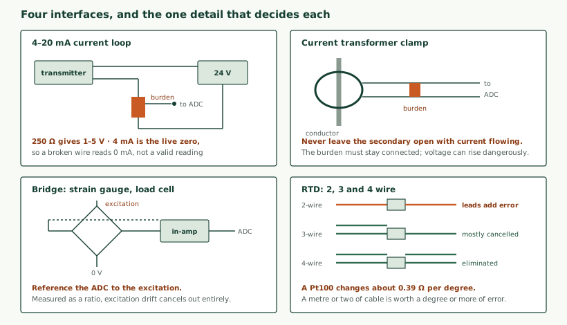
The 4-20 mA current loop

A scheme from the 1950s that remains the default for analogue process signalling, for two reasons that have not been improved upon.

Current is immune to cable resistance. A voltage signal sent down a hundred metres of cable arrives smaller, and by an amount that varies with temperature and cable batch. A current signal arrives identical, because the transmitter adjusts its output voltage to maintain the current regardless of what is in the way.

The live zero distinguishes zero from broken. A measurement at the bottom of its range reads 4 mA. A cut wire reads 0 mA. With a 0-20 mA scheme, or a voltage scheme, those two are the same reading, and a failed sensor is indistinguishable from a genuine minimum. This is the same principle as the quality indication discussed in edge gateways, implemented in analogue.

Designing the receiving end

The receiver converts current to voltage through a burden resistor, and the details matter more than the simplicity suggests.

• Value. 250 Ω gives 1-5 V, which suits most converters. Larger gives more signal and consumes more of the loop’s voltage budget.
• Tolerance and temperature coefficient. The resistor is directly in the measurement path, so its error is your error. A 1% resistor caps accuracy at 1% regardless of the converter; 0.1% with a low temperature coefficient costs little more.
• Protection. A field wire that meets 24 V, or worse, should not destroy the input. Series resistance, clamping diodes and a fuse or resettable device are cheap compared with a failed input on an installed product.
• Filtering before the converter. Long field cables collect interference. A low-pass filter matched to the signal bandwidth belongs before the converter, not after in software — once aliased, the damage cannot be undone.
• Isolation. Where loops come from different areas, ground potential differences drive currents through the measurement path. Isolated inputs remove a whole class of problem and cost more.
• Common-mode range. A differential input has limits on how far its inputs may sit from its own ground, and long runs in an industrial plant can exceed them.

The loop voltage budget

A calculation frequently skipped, which produces installations that work until a cable is extended. The supply voltage must cover the transmitter’s minimum operating voltage, the burden resistor’s drop, the cable resistance drop, and anything else in series such as a barrier or an indicator.

With a 24 V supply, a transmitter needing 12 V, a 250 Ω burden dropping 5 V at full scale, and a couple of volts in cable and accessories, the budget is adequate but not generous. Adding a display in the loop, or a hundred metres of thin cable, can take it below what the transmitter needs — at which point the reading goes non-linear at the top of the range, which presents as a strange calibration problem rather than an obvious fault.

Two-wire loop-powered transmitters have a related constraint at the sending end: the device must run on under 4 mA, since that is the current at zero signal. That is a real limit on what a loop-powered device can do, and it is why such transmitters are simple and why anything needing more power uses separate supply wiring.

Current transformers

A clamp-on current transformer is the standard way to measure alternating current without breaking the conductor, which makes it the natural choice for retrofit energy monitoring.

It is a transformer whose primary is the conductor passing through it. The secondary carries a proportional current, and a burden resistor converts that to a voltage.

• Sizing. Choose for the actual current, not the breaker rating. A 200 A CT measuring a 15 A load uses a small part of its range and resolves poorly.
• Saturation. Exceed the rating and output stops rising proportionally, which under-reads exactly when consumption is highest.
• Phase error. A CT introduces a small phase shift, which matters for power measurement because real power depends on the phase relationship. For energy measurement rather than current measurement, a CT specified for metering is not the same as one specified for protection.
• Position. One conductor through the aperture. Two cancels. Proximity to other conductors affects accuracy.
• Direct current is invisible. A CT works on changing fields. For DC, use a Hall-effect device or a shunt.

Where current is used as a proxy for machine behaviour — cycle detection, load estimation, the signature analysis described in condition monitoring — sampling rate matters as much as accuracy. Detecting a cycle boundary needs only a few samples a second; analysing a current signature for rotor faults needs enough bandwidth to resolve sidebands around the supply frequency, which is a different converter and a different anti-alias filter.

Bridges: strain gauges and load cells

A resistance bridge converts a very small resistance change into a small differential voltage. Load cells, pressure sensors and strain gauges all work this way, and the signal is genuinely tiny — a full-scale output of a few millivolts per volt of excitation means a 10 V excitation gives perhaps 20 mV at full load.

That smallness drives everything about the circuit.

What a bridge interface has to get right

Element	Requirement	Consequence of getting it wrong
Excitation stability	Stable, or measured ratiometrically	Excitation drift appears directly as signal
Ratiometric reference	Converter referenced to the excitation	Reading drifts with temperature and supply
Amplifier offset drift	Low-drift instrumentation amplifier	Zero wanders; recalibration never sticks
Common-mode rejection	High; the signal sits on half the excitation	Noise on excitation appears in the reading
Sense lines	6-wire connection for long cable	Cable resistance reduces excitation at the cell
Filtering	Matched to the mechanical bandwidth	Vibration aliases into apparent load changes
Shield and ground	Shield connected at one end only	Ground loop injects current into the measurement

The ratiometric point is the single most valuable idea here. If the converter’s reference voltage is derived from the bridge excitation rather than from an independent reference, then the measurement becomes a ratio of output to excitation. Any drift in excitation — temperature, supply variation, ageing — affects both equally and cancels exactly. This costs nothing beyond arranging the reference correctly, and it removes the largest error source in most bridge measurements. Designs that use a separate precision reference for the converter while the excitation drifts are doing more work for a worse result.

Sense lines matter once cable is involved. Excitation current flowing through cable resistance means the voltage at the cell is lower than at the supply, and it changes with temperature. A six-wire connection adds a pair that measures the voltage actually at the cell, carrying no current and therefore no drop, and the system uses that as the reference. For a load cell at the end of ten metres of cable this is the difference between a calibration that holds and one that moves with the seasons.

Temperature: RTDs and thermocouples

The two dominant industrial temperature sensors have opposite characteristics, and the interface differs accordingly.

RTD against thermocouple

	RTD, e.g. Pt100	Thermocouple
Principle	Resistance changes with temperature	Voltage from a junction of dissimilar metals
Signal	Resistance, needs excitation current	Tens of microvolts per degree; self-generating
Accuracy	Higher, more stable over time	Lower, drifts with contamination and ageing
Range	Moderate, to a few hundred degrees	Very wide, to well over a thousand
Response	Slower, larger mass	Fast, can be very small
Interface problem	Lead resistance	Cold junction compensation
Cable	Ordinary copper	Matching extension cable required

RTD lead resistance

A Pt100 reads 100 Ω at zero degrees and changes about 0.39 Ω per degree. Cable has resistance, and in a two-wire connection that resistance adds directly to the measurement: two ohms of lead is roughly five degrees of error, and it changes as the cable warms.

Three-wire adds a conductor allowing the instrument to measure and subtract the lead resistance, cancelling most of the error provided the leads are matched. Four-wire passes excitation through one pair and measures voltage through another carrying no current, eliminating lead resistance entirely.

The practical position: three-wire is adequate for most industrial measurement and is what most transmitters expect. Four-wire is worth it for precision work, long runs, or where cable temperature varies widely. Two-wire is acceptable only for short leads where a degree or two does not matter — and worth avoiding simply because somebody will extend the cable later without realising what it does.

One more consideration: excitation current heats the element. A milliamp through 100 Ω is only a fraction of a milliwatt, but in still air with a small sensor it produces measurable self-heating. Low excitation, or pulsed excitation with measurement only during the pulse, avoids a systematic error that calibration will not catch.

Thermocouple cold junctions

A thermocouple does not measure temperature. It generates a voltage proportional to the difference between its measuring junction and the point where its wires connect to something else — the cold junction, usually the instrument’s terminals.

So the instrument must know its own terminal temperature and add it. That measurement is the cold junction compensation, and its accuracy bounds the whole system: an error of a degree at the terminals is an error of a degree in every reading, regardless of the thermocouple’s quality.

• Measure at the terminals, in good thermal contact, not somewhere else on the board that may be warmer.
• Watch for gradients. A board with a regulator dissipating heat near the terminals has a gradient across them, and the two terminals of one channel at different temperatures introduce an error the compensation cannot see.
• Use matching extension cable. Ordinary copper creates another junction of dissimilar metals — another thermocouple, uncompensated, in series with yours.
• Amplify carefully. Tens of microvolts per degree is small enough that amplifier offset drift is a direct temperature error.
• Consider isolation. Grounded thermocouples on plant equipment can differ in potential, and a shared-ground multi-channel input will read the difference.

The other interfaces you will meet

Four interfaces cover most industrial measurement, but a handful of others appear regularly enough to be worth knowing where they differ.

Other common sensor interfaces

Interface	Used for	The thing to watch
Digital sensors on I²C or SPI	Temperature, humidity, pressure, inertial	Short range only; bus loading and pull-up sizing; no isolation
Pulse and frequency inputs	Flow meters, encoders, counters	Debouncing, missed counts at speed, and what happens across a power cycle
IEPE / constant-current	Accelerometers for vibration	Supplies bias current on the signal line; needs AC coupling and a settling time
Piezoelectric, charge output	High-temperature vibration, force	Charge amplifier required; cable capacitance affects the reading
Potentiometric	Position, valve feedback	Wear at one spot; measure ratiometrically against the supply
Voltage output, 0-10 V	Building services, drives	Cable drop over distance; no broken-wire detection
Switch and contact inputs	Limits, alarms, status	Contact bounce, wetting current, and the long cable acting as an aerial

Two of these deserve a note. IEPE accelerometers are the standard for the condition monitoring described in condition monitoring for rotating equipment, and their interface has a specific characteristic: the same conductor carries both the supply current and the signal, so the input must provide a constant current, block the DC bias, and allow time for the bias to settle after power-up before readings mean anything. A system that starts sampling immediately records the settling transient as a dramatic vibration event.

Pulse inputs look trivial and produce a recurring class of dispute, because they usually feed a total — of volume, energy or production — that somebody reconciles. The questions that matter are whether counts survive a power cycle, whether the input can miss pulses at maximum rate, and whether contact bounce is being counted as multiple pulses. A totaliser that resets on power loss, or double-counts a bouncing contact, produces a figure that disagrees with a manual check and is then blamed on the meter.

Protecting the input

Field wiring meets things it should not. During commissioning, wires get connected to the wrong terminals; in service, cables take transients from switching and lightning. An input that does not survive this is a service call.

• Series resistance limits fault current and is the cheapest element in the chain. It must be chosen against its effect on the measurement.
• Clamping to the supply rails, using devices rated for the energy expected rather than only the voltage.
• Transient suppression sized for the environment — a cable running outdoors between buildings faces a different threat from one inside a cabinet.
• Reverse polarity tolerance, because the wires will be swapped at some point.
• Sustained overvoltage survival. Clamping a transient is not the same as surviving 24 V applied indefinitely to a 5 V input, which is the usual commissioning error.
• Fail safely. Where protection eventually fails, it should fail in a way that is detectable rather than producing a plausible wrong reading.

The last point is the one that distinguishes a well-designed industrial input. A destroyed input reading a steady mid-scale value is worse than one reading obviously nothing, because the first is trusted. Designing so that failure produces an out-of-range or clearly invalid result, and checking for that in firmware, converts a silent fault into a visible one.

A short glossary

Terms used in this article

Term	Meaning
Burden resistor	The resistor converting a current signal into a voltage. Its accuracy is directly your accuracy.
Live zero	Using 4 mA rather than 0 for the bottom of the range, so a broken wire is distinguishable from a genuine minimum.
Loop-powered	A transmitter drawing its operating power from the same loop that carries the signal, so it must run on under 4 mA.
Ratiometric	Measuring a signal as a proportion of its own excitation, so excitation drift cancels.
Sense lines	Extra conductors measuring voltage at the sensor, carrying no current and therefore no voltage drop.
Cold junction	Where thermocouple wires meet the instrument. Its temperature must be measured and added.
Self-heating	Warming of a resistance sensor by its own excitation current, producing a systematic error calibration will not catch.
Effective resolution	The bits that carry signal rather than noise. Always fewer than the nominal figure.
Common-mode rejection	An amplifier’s ability to ignore what is common to both inputs. What makes small differential signals usable.
Anti-alias filter	Analogue filtering before the converter. Must be analogue: once aliased, the damage is not reversible in software.
IEPE	An accelerometer interface carrying supply current and signal on one conductor. Needs AC coupling and settling time.
Wetting current	A minimum current through a switch contact, sufficient to break through surface oxidation and make reliable contact.

Choosing the converter

The analogue-to-digital converter is chosen early and frequently on the wrong criterion. More bits is the obvious metric and rarely the useful one.

What actually matters in converter selection

Property	Why it matters	Common mistake
Effective resolution	The bits that carry signal rather than noise	Quoting nominal bits; the last few are frequently noise
Architecture	Sigma-delta for slow precise work, successive approximation for fast	Using a fast converter for a slow measurement and fighting noise
Integrated amplifier	Removes an external stage and its drift	Building a discrete front end that performs worse
Reference	Sets absolute accuracy, or is made irrelevant by ratiometric design	A precision reference where ratiometric would be better and cheaper
Input impedance	Must not load the source	Switched-capacitor inputs drawing charge from a high-impedance sensor
Rejection of mains frequency	Sigma-delta converters can notch 50 or 60 Hz	Not configuring it, then filtering in software afterwards
Channel count and multiplexing	Settling between channels takes time	Assuming instant switching; adjacent channels bleed into each other

Two points deserve expansion. Mains rejection is free precision. A sigma-delta converter whose sampling is arranged to integrate over an exact number of mains cycles rejects mains interference almost completely. Configuring that correctly removes the dominant noise source in most industrial measurement without a single component, and it is regularly left at a default that does not align with local mains frequency.

Multiplexer settling causes a specific confusing symptom. Switching between channels with different voltages requires the input to settle, and if the converter samples too soon each channel carries a little of the previous one. This presents as channels influencing each other, is easily mistaken for a wiring fault, and is fixed by allowing settling time or by adding a buffer.

Resolution against accuracy, again

A 24-bit converter does not give 24 bits of usable measurement. Noise in the converter, the reference, the amplifier and the wiring sets a floor, and bits below it describe noise in fine detail. Effective resolution — sometimes given as noise-free bits — is the honest figure, and it drops as gain and sample rate rise.

The practical consequence is that averaging genuinely helps, at a known rate: averaging four samples improves the noise floor by about one bit, sixteen by two, and so on, provided the noise is random. What averaging cannot fix is systematic error, which is why a stable, well-referenced, well-filtered measurement at 16 bits is worth more than a noisy 24-bit one.

Isolation, and when it is worth the cost

Isolation breaks the electrical connection between the measurement and the rest of the system while passing the signal. It costs money, board space and power, and it solves problems that are otherwise close to unsolvable.

• Ground potential differences. Two points in a plant a hundred metres apart are not at the same potential, and the difference can be volts, varying with plant load. Without isolation that difference appears across the measurement.
• Safety. Where the measurement is at or near mains potential, isolation is what keeps the low-voltage side safe to touch and is generally a requirement rather than a design choice.
• Channel-to-channel interaction. Grounded thermocouples on different machines will differ in potential; without per-channel isolation the readings interact.
• Surge protection. Isolation limits how far damage propagates when a field cable takes a transient.
• Noise breaking. Removing a ground loop removes the current circulating in it.

The decision is usually straightforward: isolate where the field cable leaves the cabinet, where mains potential is involved, or where multiple channels connect to separately grounded equipment. Within a single enclosure on a single ground, it is generally unnecessary. Channel-to-channel isolation costs considerably more than bulk isolation of a whole group, so it is worth being clear whether the problem is between the field and the system or between channels.

Powering the analogue side

The supply feeding a measurement circuit is part of the measurement, and treating it as a solved problem is a common way to lose the last few bits of resolution.

Switching regulators are efficient and produce noise at their switching frequency and its harmonics, which lands directly in the analogue supply. Three arrangements address it, in increasing order of effort: filtering the switcher’s output adequately, following it with a low-dropout linear regulator to clean up the last part, or running the analogue section from a separate quiet supply entirely. For anything above about twelve usable bits, the linear post-regulator is usually worth its small inefficiency.

Two further points. Reference noise is signal noise, so a converter’s reference deserves its own careful decoupling rather than sharing a noisy rail. And watch the switching frequency against the sample rate: a regulator switching close to a multiple of the sampling rate produces a slow beat that appears as a drifting reading and is remarkably hard to diagnose, because it looks like a real process variation rather than interference.

Grounding and shielding

More measurement problems come from grounding than from any component choice, and the rules are simple enough to state, though applying them requires thinking about where current actually flows.

• Separate analogue and digital returns, joined at one point, usually at the converter. Digital return currents are full of switching edges and must not flow through the analogue reference.
• Know the return path. Current returns by the path of least impedance, which at high frequency is directly under the outgoing track. A break in the plane beneath a signal forces a detour, and that loop radiates and picks up. This is the same principle covered in EMC and compliance design.
• Shields at one end only for signal cables — normally the receiving end. Connected at both, the shield becomes a conductor between two grounds and carries the current it was meant to exclude.
• Keep the sensitive reference clean. The converter’s reference and its ground deserve the same care as the signal; noise there appears as signal.
• Route away from switching. Analogue tracks running near a switching regulator or its inductor pick up what that node is doing. A few millimetres of separation is free at layout.

A useful discipline when a measurement is noisy: rather than reaching for a better component, trace where return current flows and where the shield terminates. The answer is usually there.

Proving the front end before trusting it

An analogue front end can be wrong in ways that look entirely plausible, so it is worth verifying deliberately rather than assuming a reasonable-looking number is correct. A short bench sequence settles most of it.

1. Measure the noise floor with the input shorted. This is the best the system will ever do, and it tells you how many bits are real. If it is worse than expected, nothing downstream will be better.
2. Apply a known input and check the absolute reading. A calibrator, a precision resistor, or a reference cell. Gain and offset errors show immediately.
3. Sweep the full range. Non-linearity and clipping appear at the extremes, which is exactly where a bench test using mid-range values never goes.
4. Change the temperature. A heat gun and a freezer spray, with readings recorded. Drift that takes months to notice in the field appears in minutes.
5. Vary the supply. Within its tolerance, the reading should not move. If it does, the measurement is not properly referenced.
6. Test with the real cable. Eighty metres of field cable behaves differently from a bench lead, and this is where lead resistance and interference actually appear.
7. Inject interference deliberately. Switch a contactor nearby, run a radio handset near the cable. Better to find the susceptibility here than at formal testing.
8. Check the failure modes. Disconnect the sensor, short it, reverse it. Confirm each produces something recognisable as a fault rather than a believable reading.

Steps 1 and 8 are the ones most often skipped and the most informative. The noise floor tells you what the design is actually capable of, independent of any claim on a datasheet. The failure behaviour determines whether a broken sensor will be noticed in a week or in a year.

Calibration and what the circuit must allow

Every analogue chain has gain and offset errors. Calibration corrects them, and whether it can be done well depends on decisions made in the circuit.

• Provide a way to inject a known input, or at least to measure a known reference through the same path. A chain that cannot be checked without dismantling will not be checked.
• Store coefficients in the device, not in a spreadsheet. A board that carries its own calibration can be replaced without recalibrating the system.
• Record when and against what. A reading is only interpretable later if its calibration status is known, as covered in process and environmental monitoring.
• Separate gain and offset. Two-point calibration corrects both; one-point corrects only offset and is frequently all that field conditions allow.
• Consider temperature. Where drift matters, measuring board temperature alongside the signal allows correction, and it costs almost nothing to add a sensor.

The last is worth doing routinely in industrial products. A temperature sensor near the analogue front end costs little, and having a record of it converts an unexplained drift into a correctable one — or at least into a diagnosable one.

A worked example

A machine builder wants to add load monitoring to a press: four load cells, a cabinet-mounted controller, cable runs of around eight metres, readings used both for a live display and for recorded quality evidence.

What the requirement implies, working through the article:

• Ratiometric measurement, because the readings feed quality records and must not drift with the cabinet temperature.
• Six-wire connection to each cell, because eight metres of cable carrying excitation current has enough resistance to move the calibration as it warms.
• A sigma-delta converter with integrated amplifier, configured to reject the local mains frequency. Four channels, with settling time allowed between them.
• Filtering matched to the mechanical event. A press cycle has a defined duration; anything faster is vibration, and letting it alias would produce apparent load variation that is not real.
• Shields terminated at the cabinet only. The cells are on the machine frame, which is grounded elsewhere.
• Board temperature recorded alongside every reading, because the quality use means drift must be explicable.
• A defined calibration route: a documented two-point procedure with coefficients stored on the board, so a controller swap does not invalidate the records.
• Protection on every field input, since a wiring error during installation is a question of when.

Almost none of this concerns which amplifier or converter to buy. The decisions that matter are about referencing, cable configuration, filtering and where shields terminate — and all of them are free at design and expensive afterwards.

What usually goes wrong

• Non-ratiometric bridge measurement. The commonest cause of load cell readings that drift with temperature.
• Two-wire RTDs on long cable. Several degrees of error that varies with the weather.
• Cold junction sensor in the wrong place. Compensating for a temperature the terminals do not have.
• Burden resistor with poor tolerance. Caps system accuracy below what everything else could deliver.
• No anti-alias filter. Interference folds into the signal band and cannot be removed afterwards.
• Unprotected field inputs. A wiring error during commissioning destroys the input, and commissioning is when wiring errors happen.
• Shields grounded at both ends. Creates a loop that injects the noise the shield was meant to exclude.
• CT sized for the breaker. Poor resolution across the range actually used.

The pattern across these is that almost none is a component selection problem. They are arrangement problems — what is referenced to what, where a sensor sits, how a shield is terminated — and they are why a circuit that simulates perfectly can measure poorly.

Buying the front end instead of designing it

Not every project should design an analogue front end. Signal-conditioning modules, DIN-rail transmitters and integrated measurement chips exist, and for low volumes they are frequently the right answer.

• DIN-rail conditioners convert almost any sensor to a standard signal, with isolation included. Expensive per channel, need cabinet space, and require no development at all.
• Integrated measurement devices — a single chip handling excitation, amplification and conversion for a bridge or an RTD — remove most of the difficulty described in this article for a modest component cost. For many products these are simply the correct choice.
• Transmitters at the sensor convert to 4-20 mA at the measurement point, so only a robust current signal travels, and the difficult analogue work becomes somebody else’s problem.
• Custom design earns its place at volume, where unusual requirements apply, or where the integrated options do not reach the needed performance.

The honest framing is a volume and risk calculation. Below a few hundred units, the development effort and the risk of a subtle analogue problem usually outweigh the per-unit saving; above a few thousand, the economics reverse. Where a requirement is ordinary — an RTD, a load cell, a current loop — an integrated part designed for exactly that job will generally beat a discrete design on cost, board area and time, and we would say so rather than quote for the design work.

How we help with this

We design interface circuits for the measurement actually required: isolation, protection, filtering, amplification and converter selection, along with the layout and grounding that determine whether the circuit performs as intended.

We would want to know the cable lengths, the environment, the required accuracy and what the measurement will be used for before designing anything. Those determine the circuit more than the sensor does, and an interface designed for a benchtop and installed at the end of eighty metres of cable in a plant room is the usual reason a measurement disappoints.

Related reading: sensor selection and signal conditioning for choosing what to measure, PCB design in practice for the layout, EMC and compliance design for interference, process and environmental monitoring for calibration over a system’s life, and condition monitoring for what these measurements support. For the wider picture, what industrial IoT actually is.

If you take one thing away

In every interface described here, the decisive detail is an arrangement rather than a component: what the converter is referenced to, how many conductors reach the sensor, where the cold junction is measured, where the shield terminates. None of these appears in a parts cost, and each determines whether the measurement holds up in the field.

Which is why a design that simulates beautifully can measure poorly, and why a front end should be judged by its noise floor with the input shorted and its behaviour when the sensor is disconnected — two measurements that take minutes and tell you more than any datasheet.

Questions we are asked about this

Common questions

What clients ask before starting

Why is 4-20 mA still used?

Because current is immune to the voltage drop that defeats voltage signalling over long cable runs, and because the live zero at 4 mA distinguishes a genuine zero reading from a broken wire. Those two properties have not been improved on for long analogue runs in electrically noisy environments, which is why a signalling scheme decades old remains the default in process plant.

What size burden resistor should we use?

250 ohms is the usual choice because it converts the 4-20 mA span into a convenient 1-5 V. The value is a trade-off: larger gives more signal but consumes more of the loop voltage budget, which limits how much cable and how many devices the loop can carry. Tolerance and temperature coefficient matter more than people expect, since the resistor is directly in the measurement path.

Do we need 3-wire or 4-wire for an RTD?

It depends on lead length and the accuracy you need. A Pt100 changes about 0.39 ohms per degree, so a couple of ohms of lead resistance is several degrees of error in a 2-wire connection. Three-wire cancels most of it and is adequate for the majority of industrial measurement; four-wire eliminates it and is worth using for precision work or long runs.

Why does our load cell reading drift with temperature?

Several possible causes, but the most common is that the measurement is not ratiometric. If the analogue-to-digital converter uses its own reference rather than the bridge excitation, any drift in the excitation appears directly as a signal change. Referencing the converter to the excitation makes the measurement a ratio, and excitation drift cancels out entirely.

Can we measure current with a simple shunt instead of a CT?

Yes for low-voltage direct-current work, and it is usually the better choice there. For mains alternating current a shunt puts your circuit at line potential, which brings isolation requirements and safety considerations that a clamp-on current transformer avoids entirely. The CT also installs without breaking the conductor, which frequently decides it on retrofit work.

What is cold junction compensation?

A thermocouple measures the difference between its measuring junction and the point where its wires meet the instrument, so the instrument must know its own terminal temperature to calculate the absolute reading. That measurement is the cold junction compensation, and its accuracy limits the whole measurement — a thermocouple system is only as good as the temperature sensor at its terminals.

Why is our signal noisy despite good components?

Noise is far more often a layout and grounding problem than a component one. The usual causes are a ground arrangement that puts return currents through the measurement reference, long unshielded runs to high-impedance inputs, and inadequate filtering before the converter. Replacing the amplifier with a quieter one rarely helps when the noise arrives through the wiring.

What do you actually provide?

Interface circuit design for the measurement you need, including isolation, protection, filtering and converter selection, plus the layout and grounding that decide whether it performs as designed. We would want to know the cable lengths, the environment and the accuracy actually required before designing anything, because those determine the circuit more than the sensor does.

Start a conversation

What are you trying to measure, and how far away is it?

Tell us the sensor, the cable length, the environment and the accuracy you actually need. Those four decide the circuit more than anything on a datasheet.

Leave empty

Your name *

Email address *

Company

Country *

What are you working on? * I agree that iTechGeeks may use these details to respond to my enquiry. Privacy policy. Send enquiry ↗

Prefer email? Write to info@itechgeeks.in