
Sensor selection and signal conditioning: the chain that decides your data
Sampling, aliasing, conditioning, noise, mounting and calibration. Everything downstream inherits the quality of what you captured, and no processing puts back what was lost.
In short
- Most measurement problems that surface late were created at the start, when someone chose a sensor from a catalogue and a sampling rate from habit.
- Information lost before the converter cannot be recovered by any amount of processing afterwards.
- Resolution is not accuracy. A 24-bit converter on a poorly designed front end produces very precise wrong numbers.
- Mounting and placement frequently matter more than which sensor you bought.
- Design in a way to tell a failed sensor from a stable process. The two look identical otherwise.
The quiet decision that determines the project
Connected product and monitoring projects tend to fail in a recognisable way. Everything works in development, the data looks plausible, and then someone asks a question the data cannot answer, or an analysis produces a result nobody believes. Tracing it back usually leads to a decision made in the first fortnight: which sensor, mounted where, sampled how fast.
That decision sets a ceiling. No amount of firmware, cloud processing or machine learning recovers information that was never captured. If the sampling rate missed the phenomenon, the information is not in the data. If the sensor was measuring the wrong thing, or the right thing in the wrong place, the record is of something else. If the front end saturated on peaks, the peaks are gone.
This article is about getting that part right, because it is where the leverage is and it is consistently the least discussed part of an IoT project.
The chain, and where error enters
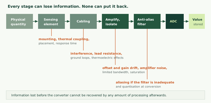
It helps to think of measurement as a chain rather than a component. The physical quantity acts on a sensing element, which produces a small electrical signal. That signal travels along a cable, gets amplified and possibly isolated, is filtered, is converted to a number, and is then processed and stored. Each stage can degrade what passes through it, and the degradation at one stage is invisible at the next.
Designing a measurement means designing the whole chain, with the constraints of each stage informing the others.
Deciding what to measure at all
Before choosing a sensor, be clear about what physical quantity actually carries the information you need. This sounds obvious and is frequently where the most expensive mistakes are made, usually by measuring the thing the question mentions rather than the thing that changes.
If you want to know whether a pump is degrading, several quantities carry that information: vibration at the bearings, the current the motor draws, discharge pressure, temperature, or the acoustic signature. They differ enormously in how easy they are to measure, how invasive the installation is, and how early the degradation appears in them.
Indirect measurement is often better than direct. Measuring motor current at the supply panel requires no modification to the machine, no process penetration, and no permit for work on pressurised equipment, while telling you a great deal about what the machine is doing mechanically. A pressure tapping would tell you something more specific and cost considerably more to install.
The useful question is therefore not “how do we measure X” but “what observable quantity changes when the thing we care about changes, and which of those is cheapest and least disruptive to observe reliably”.
Sensor types, and what each demands of the circuit
The sensing element determines what the rest of the front end must do. A few common cases, with the implications that follow.
| Quantity | Approach | Signal | What the front end must handle |
|---|---|---|---|
| Temperature | Thermocouple | Millivolts, non-linear | High gain, cold junction compensation, linearisation |
| Temperature | Resistance detector | Small resistance change | Excitation current, lead resistance compensation, self-heating |
| Temperature | Thermistor | Large resistance change | Simple divider, strongly non-linear, limited range |
| Temperature | Integrated digital sensor | Digital | Little analogue work; placement and thermal coupling become the issue |
| Vibration | Piezoelectric, constant current type | AC, wide bandwidth | Current source, AC coupling, high sample rate |
| Vibration | MEMS accelerometer | Digital or analogue | Lower bandwidth, can measure static acceleration, cheaper |
| Force and weight | Strain gauge bridge | Millivolts per volt | Bridge excitation, instrumentation amplifier, ratiometric conversion |
| Current, AC | Current transformer | Current proportional to primary | Burden resistor, isolated inherently, AC only |
| Current, AC or DC | Hall effect or fluxgate | Voltage | Isolated, offset drift with temperature |
| Current, direct | Shunt resistor | Millivolts | Amplification, and isolation if referenced to a hazardous potential |
| Pressure, level, flow | Industrial transmitter | 4-20 mA or digital | Loop supply, sense resistor, straightforward and robust |
Two points are worth drawing out of that table.
The first is that integrated digital sensors remove most of the analogue design problem, and where one exists that suits the application it is usually the right choice. What it does not remove is the physical problem: a digital temperature sensor still has to be thermally coupled to the thing whose temperature you want, and a sensor measuring the air near a bearing is not measuring the bearing.
The second is the enduring value of the 4-20 mA current loop in industrial installations. A current signal is immune to voltage drop along the cable, far more resistant to induced interference than a low-level voltage, and, crucially, allows a broken wire to be distinguished from a genuine zero, because zero current is outside the valid range. That diagnostic property is worth a great deal in installations where a silently failed sensor is dangerous.
Range, resolution and accuracy are three different things
These terms are used interchangeably in specifications and they mean quite different things.
Range is the span the system can measure without clipping. Choose it from the worst case, not the normal case: a vibration front end that saturates during a startup transient loses exactly the event you were most interested in.
Resolution is the smallest change the system can distinguish. It is set by the converter, the noise floor and the gain, and it is frequently quoted from the converter alone, which is optimistic.
Accuracy is how close a reading is to the true value. It is limited by the sensor’s own accuracy, by drift, by calibration and by everything in the chain, and it is usually far worse than the resolution.
The practical consequence is that a high-resolution converter does not produce accurate measurements. It produces very finely divided readings of whatever the front end presented to it, and if that was drifting or noisy, the extra bits describe the noise in remarkable detail.
There is also a useful distinction between accuracy and repeatability. For condition monitoring, repeatability usually matters more: you want to know whether today’s reading differs from last month’s on the same machine, and a consistent offset is harmless for that purpose. For anything being compared against a specification or another instrument, accuracy matters and calibration becomes necessary, which is the subject of process and environmental monitoring.
Bandwidth, sampling and the failure mode that produces plausible nonsense
This is the part most worth understanding properly, because getting it wrong produces data that looks entirely reasonable and is wrong.
A signal must be sampled at more than twice the highest frequency it contains. Sample more slowly and higher frequencies do not simply disappear; they are folded down and appear as lower frequencies that were never present. This is aliasing, and its defining characteristic is that the result is indistinguishable, after the fact, from real signal.
The remedy is an analogue filter before the converter that removes everything above half the sampling rate. It must be analogue and it must be before conversion, because once aliasing has occurred there is no digital process that can undo it. A digital filter applied afterwards removes the frequency band; it does not remove the corruption that was folded into it.
This has a direct consequence for condition monitoring. Early bearing degradation appears in high-frequency content, so a system sampling fast enough only for running speed and its low harmonics will miss the early warning it was installed to provide, while producing a comfortable-looking trend. Deciding the sampling rate therefore means deciding what you need to be able to see, which means understanding the phenomenon before specifying the hardware.
A cheap technique worth knowing. Sampling faster than strictly necessary and averaging groups of samples reduces random noise and can recover effective resolution beyond what the converter nominally provides. Roughly, each fourfold increase in sampling rate buys about one additional effective bit, up to the point where other error sources dominate. It costs processing rather than hardware, and it is frequently the easiest improvement available on an existing design.
What the conditioning circuit does
Between sensing element and converter sits the work that decides whether the reading is usable.
Amplification scales a small signal to match the converter’s input range. Getting this right matters in both directions: too little gain wastes converter range and resolution, too much clips on peaks. For differential signals from bridges and thermocouples, an instrumentation amplifier is the appropriate part, because it rejects the voltage common to both inputs, which is where most interference appears.
Filtering removes what you do not want before it is digitised. The anti-alias filter is mandatory; additional filtering to reject mains-frequency interference or mechanical resonances is often worthwhile. Every filter costs response time, so the trade-off between noise rejection and speed is a design decision rather than a default.
Isolation separates the measurement from the rest of the system electrically. It is necessary for safety where the measured point sits at a hazardous potential, and useful wherever the sensor and the measuring circuit have different ground references, which in industrial installations is common. Isolation costs money, board area and some performance, and is one of the more frequently omitted items that later proves necessary.
Protection keeps the circuit alive when something unexpected happens at the terminals: static discharge, an induced surge, or a miswired connection applying supply voltage to a signal input. Industrial inputs should assume all three will occur eventually.
A stable reference determines whether the measurement means the same thing next month. Converter accuracy is relative to its reference, so reference drift appears directly as measurement drift. Where the sensor is excited from the same reference used for conversion, as in a bridge measurement, the arrangement becomes ratiometric and reference drift largely cancels, which is an elegant and free improvement worth designing in.
A note on integrated sensor modules
A great deal of the analogue design described here can be avoided by buying a module that has already done it: a sensor with conditioning, conversion and a digital interface in one part, or an industrial transmitter that outputs a current loop or a digital protocol.
Where a suitable one exists, this is usually the right choice. The manufacturer has characterised the chain, handled the calibration, and taken responsibility for the performance figures. Development time falls substantially, and the risk of an analogue design problem surfacing late disappears with it.
The trade-offs are worth being explicit about. You accept the manufacturer’s choices about filtering and sampling, which may not suit your application, and those choices are frequently not fully documented. Bandwidth is often lower than a bespoke design would achieve, which matters for vibration work in particular. Unit cost is higher, which matters at volume. And you inherit a supply chain dependency on a specific part, which is a real risk over a product life measured in years.
The decision usually turns on volume and on how demanding the measurement is. For low volumes and undemanding measurements, a module is almost always correct. For high volumes, or where bandwidth, noise or power constraints are tight, a designed front end earns its development cost. Between those, it is worth pricing both.
Choosing the converter
Two families cover most industrial work and they suit different problems.
| Type | Character | Suits | Watch for |
|---|---|---|---|
| Successive approximation | Fast, low latency, easy to multiplex across channels | Vibration, current waveform, anything needing speed | Requires a proper external anti-alias filter |
| Delta-sigma | High resolution, oversamples internally, slower | Temperature, weight, pressure, precision measurement | Latency; settling time when switching channels |
| Integrated in the microcontroller | Convenient, no extra parts | Undemanding measurements | Effective resolution well below the nominal figure |
| Inside the sensor | Removes the analogue problem entirely | Where a suitable part exists | You accept the manufacturer’s conditioning choices |
The figure worth asking about is effective resolution rather than nominal bits. A converter advertised at sixteen bits may deliver meaningfully fewer usable bits once its own noise is accounted for, and the number degrades further with a noisy front end or a poor supply. Manufacturers usually publish this; it is a better basis for comparison than the headline.
Noise, and where it comes from
Noise sets the floor beneath which measurement is meaningless, and knowing which kind you have determines which remedy works.
- Thermal noise is generated by resistance and is unavoidable. It is reduced by lowering source resistance and by limiting bandwidth to what you actually need.
- Amplifier noise depends on the part and on the source impedance it sees. Matching the amplifier to the sensor rather than choosing the lowest-noise part available is the useful approach.
- Low-frequency drift matters for slow measurements, where it appears as a reading that wanders over minutes. Chopper-stabilised amplifiers exist specifically for this.
- Mains interference couples in from wiring and equipment. It is highly predictable, which makes it straightforward to reject: a filter, a differential input, or an integration time that is a whole number of mains cycles all work.
- Switching noise from power supplies and motor drives is broadband, fast-edged and the dominant nuisance in industrial environments. It is addressed through layout, filtering and physical separation. The same mechanisms decide whether a product passes emissions testing, which we cover in EMC and compliance.
- Ground loops occur when two points that should be at the same potential are not, and current flows through the signal return. This is a wiring problem with a wiring solution, most often isolation or single-point grounding.
A practical habit: measure the noise floor of the finished chain with the input shorted or with the sensor in a known stable condition. That tells you what the system can actually resolve, which is frequently worse than the specification suggested, and it gives you a baseline against which to judge later problems.
Layout, grounding and cabling
For low-level signals, the physical arrangement often matters more than the choice of components.
- Keep analogue signals short and away from switching circuits, clocks and anything with fast edges.
- Give returns an uninterrupted path. A split in a reference plane under a sensitive trace turns a careful design into an antenna.
- Use differential signalling over distance, with twisted pairs, so interference appears on both conductors and is rejected.
- Ground the shield at one end only for low-frequency measurements. Grounding both ends creates exactly the loop the shield was meant to prevent.
- Use four-wire connections for low resistances. Lead resistance is indistinguishable from the thing you are measuring otherwise, which matters for resistance thermometers and shunts.
- Watch for thermoelectric voltages. Junctions between dissimilar metals generate small voltages with temperature differences, which is significant when the signal itself is only a few millivolts.
- Route signal cables away from power cables, and cross at right angles where they must cross.
These are the details that separate a design that works on a bench from one that works next to a motor drive. Our wider hardware work is described in hardware and PCB design.
Mounting and placement
The sensing element measures what reaches it. Where it is and how it is attached therefore determine what it can possibly detect.
For vibration, mounting method sets the usable frequency range. A rigidly attached sensor transmits high frequencies faithfully; a magnetically mounted one degrades at exactly the high frequencies where early bearing degradation appears. That is acceptable for a survey and a poor choice for permanent monitoring, and the difference is invisible in the data unless you know to look for it. Location matters equally: a sensor on the bearing housing measures the bearing, while the same sensor on a guard panel nearby measures mostly the panel.
For temperature, thermal coupling and response time dominate. A sensor measuring air near a surface will lag the surface considerably and settle at a different value. Where you need surface temperature, the sensor must be thermally bonded to the surface and insulated from the surroundings.
For anything being trended over time, consistency is as important as correctness. A sensor that moves between readings makes comparison meaningless, which is a strong argument against removable mounting for permanent installations, and an argument for documenting and photographing installation positions so that a replacement goes back in the same place.
Calibration and drift
A measurement chain is trustworthy only if you know how it behaves over time and temperature.
The decisions to make early are where calibration happens, against what reference, how coefficients are stored, and how a unit is recalibrated in five years by someone who did not build it. Calibrating in manufacturing gives a known starting point; calibrating in the field accounts for installation effects; many products need both.
Temperature is the dominant drift mechanism in most designs, affecting sensor, amplifier and reference together. Where accuracy requirements are demanding, measuring the temperature of the electronics and applying correction is a well-established approach and usually cheaper than specifying components stable enough not to need it.
It is also worth deciding what happens when calibration expires or is lost. A device that silently reverts to default coefficients produces confident wrong readings; one that reports its calibration status lets the system decide how much to trust it.
Surviving the environment
A measurement that is correct on commissioning day and wrong eighteen months later has cost you more than one that never worked, because nobody noticed the transition.
- Ingress. Dust, coolant, washdown and condensation all find their way in eventually. The rating needs to match the real conditions rather than the nominal ones, and washdown in particular is far more demanding than rain.
- Condensation. Frequently overlooked, and more damaging than immersion because it occurs repeatedly inside sealed enclosures as temperature cycles. A sealed box that breathes through a small leak accumulates water. Controlled venting through a membrane is the usual answer.
- Chemical exposure. Cutting fluids, cleaning agents and process chemicals attack cable jackets, seals and connector bodies. Material compatibility should be checked rather than inferred from an ingress rating.
- Vibration fatigue. Connections that are fine in a cabinet fail on a machine. Cables need strain relief and support, connectors need retention, and solder joints carrying mechanical load will eventually crack.
- Temperature cycling. It drives drift, degrades seal performance, and works connections loose over thousands of cycles.
- Cable routing. Cables are the most commonly damaged part of a retrofit installation. They get caught, crushed, cut during unrelated work, and pulled when equipment moves. Routing them where people and machinery are not is worth the extra metres.
For long-term installations the failure rate is usually dominated by connections and cabling rather than by sensing elements. Design accordingly: fewer connectors, better strain relief, and accessible routing for the replacement that will eventually be needed.
More than one sensor
Where a measurement matters, a second one is often the cheapest way to make it trustworthy.
Redundancy means two sensors measuring the same quantity, which lets you detect that one has failed rather than merely suspecting it. A pair disagreeing is a far stronger signal than either one looking slightly odd.
Cross-checking different quantities is frequently more useful and cheaper. Motor current and vibration should tell a consistent story about whether a machine is running. A temperature that rises without a corresponding load increase is either a genuine problem or a sensor fault, and either way it warrants attention. Relationships between measurements are often more robust than any single measurement’s absolute accuracy.
Context measurements make the primary measurement interpretable. Ambient temperature explains drift. Machine state explains why vibration changed. Product type explains why current differs this week. Collecting these alongside the measurement you care about costs little and prevents a large class of false conclusions, as discussed in predictive maintenance.
Verifying a measurement design
A measurement chain should be characterised rather than assumed to work. The following are quick, and each catches a distinct class of problem.
- Noise floor. Short the input, or hold the sensor in a stable condition, and record. This tells you the smallest change the system can genuinely resolve.
- Known input. Apply a signal of known amplitude and confirm the reported value. This verifies gain, scaling and conversion arithmetic in one step.
- Frequency response. Sweep the input frequency and confirm the system responds as designed, and importantly that it rejects frequencies above half the sampling rate rather than folding them down.
- Step response. Apply a sudden change and observe settling. This reveals filter time constants slower than intended, which matters when a fast event must be caught.
- Overload recovery. Drive the input beyond range and confirm the system recovers promptly rather than sulking for seconds afterwards.
- Temperature. Measure drift across the operating range, ideally with the sensor stable and only the electronics cycling, so you know which contributes what.
- Comparison against a reference. Against a calibrated instrument, at several points across the range rather than only one.
- Soak test. Left running for days in representative conditions. Intermittent faults and slow drift only appear with time.
The output should be a written characterisation: this is the noise floor, this is the usable bandwidth, this is the drift per degree, this is what it was compared against. That document is what later allows anyone to judge whether an unexpected reading is a real event or a limitation of the instrument.
A short glossary
| Term | Meaning |
|---|---|
| Aliasing | Frequencies above half the sampling rate appearing as lower frequencies that were never present. Indistinguishable from real signal afterwards. |
| Anti-alias filter | An analogue filter before the converter removing everything above half the sampling rate. Cannot be replaced by digital filtering. |
| Effective resolution | The usable resolution once noise is accounted for. Always less than the converter’s nominal bit count. |
| Ratiometric measurement | Exciting a sensor from the same reference used for conversion, so reference drift largely cancels. |
| Common-mode rejection | An amplifier’s ability to ignore voltage present equally on both inputs, which is where most interference appears. |
| Instrumentation amplifier | An amplifier built for small differential signals, with high common-mode rejection and high input impedance. |
| Cold junction compensation | Correcting a thermocouple reading for the temperature where it connects to the measuring circuit. |
| Four-wire measurement | Separate pairs for excitation and sensing, so lead resistance does not appear in the reading. |
| Burden resistor | The resistor converting a current signal into a voltage the converter can read. |
| Noise floor | The level of the system’s own noise, beneath which changes cannot be distinguished. |
| Oversampling | Sampling faster than strictly required and averaging, to reduce noise and improve effective resolution. |
| Settling time | How long the chain takes to report a correct value after a change, set largely by filtering. |
Knowing when the sensor has failed
This is routinely omitted and it is one of the highest-value features a measurement system can have.
The most dangerous failure is a sensor that reports its last value indefinitely. On a dashboard it looks like an exceptionally stable process. Every analysis built on it continues confidently. It can persist for months.
Detectable conditions include a value that has not changed at all for longer than physically plausible, a reading pinned at the extreme of range, a rate of change that exceeds what the physical process can produce, a value outside the physically possible, a current-loop reading outside the valid band indicating a broken wire, and disagreement between sensors that should track each other.
Each of these is straightforward to implement and each should set a quality indicator that travels with the data rather than being resolved silently, and preserved through the pipeline as described in cloud backends and dashboards. A value flagged as suspect can be excluded from an average; a value silently substituted cannot be reasoned about later.
Diagnosing a measurement that looks wrong
Often the work is not designing a new chain but working out why an existing one is producing something implausible. The symptoms narrow the cause down quickly.
| Symptom | Likely causes | First check |
|---|---|---|
| Reading is stable but wrong by a constant amount | Offset error, calibration, wrong scaling constant | Apply a known input and compare |
| Wrong by a proportion that grows with the value | Gain error, wrong reference, incorrect burden or divider | Check at two points across the range |
| Wildly wrong, often by a factor or negative | Byte or word order, signed and unsigned confusion, wrong register | Read a value you can verify independently |
| Noisy, with a strong periodic component | Mains interference, switching supply, drive harmonics | Look at the frequency of the noise; it usually names the source |
| Noisy, broadband | Poor grounding, high source impedance, inadequate filtering | Measure the noise floor with the input shorted |
| Drifts slowly over hours | Temperature, reference drift, self-heating | Log alongside ambient temperature |
| Jumps between two values | Intermittent connection, loose terminal, cable damage | Move the cable and watch |
| Perfectly stable, never changes | Failed sensor holding its last value, or a frozen acquisition | Force a change and confirm it is seen |
| Plausible but wrong frequencies present | Aliasing from inadequate anti-alias filtering | Sample faster and compare; the frequencies will move |
The last row is worth dwelling on, because it is the only one whose symptom is that the data looks entirely reasonable. If an aliased component is present, raising the sampling rate changes the frequency at which it appears, whereas a genuine signal component stays where it is. That test takes minutes and resolves a question that can otherwise consume weeks of analysis.
A general principle for this kind of diagnosis: work from the physical end. Confirm the sensor is seeing what you think, then the cabling, then the front end, then the conversion, then the arithmetic. Starting at the software end and working backwards is tempting because it is the accessible end, and it is usually the wrong end.
Three worked situations
Bearing condition on a motor
The requirement is early detection, which means high-frequency content, which sets the sampling rate and rules out the slower converter families. A piezoelectric accelerometer, rigidly mounted on the bearing housing, with a current-source front end, AC coupling, a proper anti-alias filter and a fast converter. Alongside it, motor current for load and speed context, because a vibration spectrum is difficult to interpret without knowing what the machine was doing. Processing at the edge to extract features rather than transmitting raw waveform continuously, as discussed in edge AI on microcontrollers.
Temperature across a process vessel
Accuracy and stability matter; speed does not. Resistance thermometers with four-wire connections to eliminate lead resistance, a delta-sigma converter with integration timed to reject mains interference, ratiometric excitation so reference drift cancels, and isolation because the vessel and the electronics have different ground references. Sampling every few seconds is ample. The engineering effort goes into stability and into thermal coupling at the sensing point rather than into bandwidth.
Energy monitoring on a distribution board
Current transformers around the supply conductors, which are inherently isolated and require no electrical modification, with a burden resistor sized to match the converter range at the largest expected current including startup surge. Simultaneous voltage measurement if real power rather than apparent current is needed, which adds an isolation requirement. Sampling fast enough to capture the harmonic content that drives equipment produces, rather than assuming a clean sinusoid, because in a plant full of drives that assumption is usually wrong.
Mistakes worth avoiding
- Choosing the sampling rate for convenience. It should follow from the phenomenon.
- Omitting the anti-alias filter because a digital filter is planned. It does not work.
- Sizing range for normal operation. Transients clip, and transients are interesting.
- Assuming converter bits are usable bits. Effective resolution is the real figure.
- Grounding shields at both ends on low-frequency measurements.
- Two-wire connections to resistance thermometers where lead resistance matters.
- Magnetic mounting left in place permanently. Fine for surveys, unreliable for trending.
- No sensor fault detection. A frozen reading looks like a stable process forever.
- Never measuring the noise floor. You do not know what the system can resolve until you do.
How we help
- Measurement strategy. Working out what to measure to answer your question, including cases where a cheaper indirect measurement does the job better.
- Sensor evaluation. Candidates assessed against range, bandwidth, environment, availability and cost, tested on the real signal where feasible rather than compared on paper.
- Front-end design. Amplification, filtering, isolation, protection, reference and converter selection, laid out with the analogue constraints respected.
- Acquisition firmware. Sampling, timing, oversampling and digital filtering matched to the analogue design. See embedded firmware development.
- Verification. Measuring the noise floor and real performance of the finished chain, so you know what your data is worth.
- Calibration approach. Practical and repeatable in production and in the field.
- Diagnosing existing measurements. Where data already exists and looks wrong.
The service page for this work is sensor selection and signal conditioning. Where the equipment is already installed and has no interface, legacy machine retrofit covers the installation side.
Where the budget actually goes
The cost distribution in measurement work is consistently different from what people expect, which matters when scoping a project.
The sensing element is rarely the largest item. Even good industrial sensors are modest against the cost of everything around them, and choosing a cheaper sensor to save money usually costs more elsewhere in compensation, calibration or rework.
Installation dominates for retrofit work. Access, mounting, cable routing, panel work by a qualified person and any production window required routinely exceed the hardware by a wide margin.
Characterisation is real engineering time. Establishing noise floor, bandwidth, drift and comparison against a reference is a proper piece of work, and skipping it is how projects end up with data nobody can defend.
Diagnosing an existing bad measurement can cost more than designing a new one, because the investigation has to eliminate possibilities in sequence and each elimination may require access to the installation.
The practical implication is that spending a little more on the measurement design at the start is almost always cheaper than the alternative, because everything downstream depends on it and the cost of discovering a problem rises steeply with how late it is found.
If you take one thing away
Every other part of a monitoring or connected product system can be changed later. Firmware can be updated, dashboards redesigned, analysis reworked, models retrained. The measurement chain is the one part whose mistakes are permanent, because the data it produced is the only record you will ever have of what happened.
That asymmetry is the argument for spending disproportionate care on it. Decide what physical quantity carries the information. Sample fast enough to see it, with a real anti-alias filter. Design the front end for the worst case rather than the typical one. Mount it consistently and document where. Measure the noise floor so you know what the numbers mean. And build in a way to tell a failed sensor from a stable process, because otherwise you will not find out for months. The circuits for the commonest industrial interfaces are covered in sensor interface circuit design. Measurement is the bottom layer of a larger structure, described in what industrial IoT actually is.
Questions we are asked about this
What clients ask before starting
Our readings are noisy. Can we fix it in software?
Partly. Filtering removes interference that sits outside the band of interest, and averaging reduces random noise. What cannot be recovered is information that was never captured, or a signal that has been corrupted by aliasing. Whether software helps depends entirely on what the raw signal contains.
How do we choose a sampling rate?
From the highest frequency you genuinely need to observe, sampled at more than twice that rate, with an analogue filter before the converter to remove everything above it. Sampling too slowly does not produce a coarse version of the signal; it produces a misleading one.
What is the difference between accuracy and resolution?
Resolution is the smallest change a system can distinguish. Accuracy is how close a reading is to the true value. A system can have very fine resolution and be consistently wrong, which is why high-resolution converters do not by themselves produce accurate measurements.
Why does sensor mounting matter so much?
Because the sensing element measures what reaches it, not what is happening elsewhere. For vibration in particular, mounting method determines which frequencies survive the path from the machine to the element, and a sensor on a guard panel may be measuring mostly the panel.
Do sensors need recalibrating?
It depends on the sensor, the accuracy required and the environment. The important thing is deciding early whether calibration happens in manufacturing, in the field or both, what reference is used, and how a unit is recalibrated years later by someone who did not build it.
Why use 4-20 mA rather than a voltage output?
Because a current signal is unaffected by voltage drop along the cable, is far more resistant to induced interference, and allows a broken wire to be distinguished from a genuine zero reading. That diagnostic property alone justifies it in many industrial installations.
How do we know a sensor has failed rather than the process changing?
By designing for it. A stuck reading, a value at the extreme of range, an implausible rate of change and a reading outside the physically possible are all detectable. A sensor that fails by reporting its last value forever is the most dangerous case, because it looks like a stable process.
Can you work out what is wrong with an existing measurement?
Usually yes. Sending us a recording of the raw signal, along with what you believe it should look like, is the most useful starting point. Many problems are diagnosable from the data before anyone visits the installation.
What are you trying to measure?
Tell us the quantity, the environment it sits in and the change you need to detect. If you already have data that looks wrong, a recording of the raw signal is the most useful thing to share.