
Edge AI on microcontrollers: what fits, and what does not
Memory budgets, inference timing, quantisation cost and the power arithmetic that decides whether a model belongs on the device at all.
In short
- Models of tens of kilobytes run comfortably on mid-range microcontrollers. Anything larger needs a different class of hardware.
- Working memory usually constrains you before model size does. Intermediate results can exceed the weights.
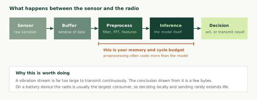
- Preprocessing often costs more cycles than the model. Feature extraction is part of the budget, not a detail.
- Measure on the target. Inference time, memory headroom and current draw on real hardware, not estimates from a datasheet.
- The usual constraint is not the model. It is whether representative data exists.
Why put a model on the device at all
Sending data to a server and deciding there is simpler to build, easier to update and usually the right answer. It is worth being clear about that, because a good deal of enthusiasm for edge AI is enthusiasm for the idea rather than for the engineering.
There are, however, situations where the cloud is genuinely the wrong place, and they are common enough in industrial and product work to matter.
- Latency. The response has to happen in milliseconds and a network round trip does not fit inside that.
- Connectivity. The device sits somewhere with intermittent, slow or metered coverage, and a system that only works when connected does not work.
- Data volume. A continuous vibration or audio stream is far too large to transmit, while the conclusion drawn from it is a handful of bytes. This is frequently the deciding factor.
- Power. On battery devices the radio is usually the largest consumer. Deciding locally and transmitting only when there is something to say can extend life by an order of magnitude.
- Data residency. The raw data should not leave the site, for commercial, contractual or regulatory reasons.
- Cost at scale. Cloud ingestion and storage priced per device per month becomes a significant recurring line across a large fleet.
What a microcontroller actually has
The constraint that shapes everything is memory, and the numbers are smaller than people coming from software development expect. A server has gigabytes. A microcontroller has kilobytes.
| Class | Typical flash | Typical RAM | Realistic for |
|---|---|---|---|
| Small, low-power core | 32-128 KB | 8-32 KB | Thresholds, filters, simple statistics; not neural networks |
| Mid-range core with DSP instructions | 256 KB-1 MB | 64-256 KB | The usual target: small classifiers, anomaly detection, keyword spotting |
| High-end core, higher clock | 1-2 MB | 512 KB-1 MB | Larger models, simple vision at low resolution, faster inference |
| Core with neural accelerator | 1-2 MB plus external | Several hundred KB plus external | Frequent inference, larger models, tighter power budgets |
| Application processor | External storage | Hundreds of MB to GB | Vision at useful resolution, larger models; different power and cost class entirely |
The step between the last two rows is the one that changes a product. An application processor running a general-purpose operating system is a different proposition in cost, power, boot time, security surface and certification effort. Where a microcontroller will do, it is usually worth the effort to make it do.
The memory budget, in detail
This is where projects get into trouble, because the model file size is the least of it.
Weights occupy flash, and after 8-bit quantisation a model of a hundred thousand parameters is roughly a hundred kilobytes. That part is easy to estimate.
Working memory is where the surprises are. Running a network requires holding intermediate results between layers, and for some architectures the largest intermediate tensor exceeds the total size of the weights. This memory is RAM, which is the scarcer resource, and it must be available simultaneously with everything else the firmware needs.
Input buffers hold the raw samples. A window of vibration data at a useful sampling rate is not small, and if you need overlapping windows you need more than one.
Preprocessing buffers hold intermediate results of feature extraction, which for frequency-domain work means at minimum the transform output and often a spectrogram built from several frames.
Everything else: the network stack, the radio driver, storage, the application logic and a stack deep enough not to overflow at the worst moment.
A practical budgeting rule. Take the quantised model size, double it to account for working memory, add the input and preprocessing buffers, and compare that against RAM after the rest of the firmware has taken its share. If the result is tight on paper, it will not fit in practice. Measure early on real hardware rather than discovering it during integration.
Inference time and the interval you have to fit inside
The model must complete well within the time between the events it processes. If you are classifying a window of data every hundred milliseconds, inference plus preprocessing must finish comfortably inside that, leaving room for acquisition, communication and everything else the device does.
Two things affect this more than people expect. Optimised kernel libraries that use the processor’s DSP instructions produce large speedups over naive implementations, frequently several fold, and using them is generally the difference between fitting and not. And integer arithmetic is substantially faster than floating point on parts without a floating-point unit, which is one of several reasons quantisation matters.
Quantisation: the compromise you will make
Models are usually trained in 32-bit floating point and deployed in 8-bit integer. The conversion reduces size roughly fourfold, often speeds inference considerably, and costs some accuracy.
| Aspect | 32-bit float | 8-bit integer |
|---|---|---|
| Size per parameter | 4 bytes | 1 byte |
| Speed on a core without an FPU | Slow | Substantially faster |
| Energy per inference | Higher | Lower |
| Accuracy | Reference | Usually slightly lower; occasionally materially so |
| Training effort | Standard | May need quantisation-aware training if post-training loss is unacceptable |
Where post-training quantisation costs too much accuracy, the usual remedy is quantisation-aware training, which simulates the reduced precision during training so the model adapts to it. This costs development time rather than runtime resources, and it frequently recovers most of the gap.
The point to hold onto is that the accuracy figure that matters is the one measured on the quantised model running on the target hardware, not the figure from the training notebook.
Preprocessing is not a detail
Raw sensor samples are rarely fed directly to a model. What happens in between, filtering, windowing, transforming to the frequency domain, extracting features, frequently consumes more processor cycles and more memory than the inference itself.
For vibration and audio work this is especially true. Computing a frequency transform on each window, then assembling features from it, is real computation on a small processor. It is also where a great deal of the eventual accuracy comes from: good features let a small model succeed where a larger model on poor features fails.
The engineering consequence is that preprocessing should be designed alongside the model rather than treated as fixed input. Often the most effective size reduction available is not compressing the network but choosing features that let a smaller network do the job.
Power, and the arithmetic that decides battery life
On a mains-powered device inference cost is usually irrelevant. On a battery device it is a design parameter.
The energy of one inference is its current draw multiplied by its duration. Run infrequently, this is negligible against the device’s sleep current. Run continuously at a high rate, it becomes the dominant consumer and the device’s active duty cycle rises accordingly.
Set against that is what inference saves. Transmitting a raw data stream costs radio energy continuously; transmitting a conclusion costs a fraction of it. For most battery devices the radio dwarfs everything else, so moving the decision on-device is usually a large net saving even accounting for the compute. The design question is how often inference must run to catch what you need, and whether a cheap screening step can decide when to run the expensive one. We cover the wider power design in battery and power engineering.
Which problems suit this
Not every task benefits from a model, and the ones that do fall into a few recognisable shapes.
| Problem | What it answers | Data needed | Typical demand |
|---|---|---|---|
| Anomaly detection | Is this different from normal? | Examples of normal only | Low; small autoencoders and statistical models fit easily |
| Classification | Which of these known states is it? | Labelled examples of each state | Low to moderate |
| Keyword or event spotting | Did the thing we care about just happen? | Labelled examples plus plenty of negatives | Moderate; continuous listening drives power |
| Regression and forecasting | What value, or what value next? | Sequences with known outcomes | Moderate |
| Vision, low resolution | Is it present, oriented correctly, obviously defective? | Labelled images across real conditions | High; often the boundary of what a microcontroller can do |
| Vision, higher resolution | Fine detail, small defects, reading | Large labelled sets | Beyond microcontrollers; needs an accelerator or an application processor |
Anomaly detection deserves particular attention in industrial work because of the data situation it requires. It needs only examples of the equipment behaving normally, which you can begin collecting immediately, whereas anything supervised needs examples of the condition you want to detect, which you may not have and cannot conjure. That asymmetry decides the first project more often than any technical consideration.
The trade-off is specificity. Anomaly detection reports that something changed; it will not tell you what, and it will flag a product changeover, a new operator or a loosened sensor mount with the same confidence as a developing fault. Interpreting its output needs context, which is why it works best combined with the operating information that explains ordinary variation.
Toolchains, briefly
A handful of ecosystems do most of this work, and the choice matters less than people expect once the constraints are understood.
| Approach | What it provides | Suits |
|---|---|---|
| Microcontroller runtimes from the major frameworks | An interpreter sized for embedded use, with a fixed memory arena and no dynamic allocation | Teams already training in that framework |
| Optimised kernel libraries for the target core | Hand-tuned implementations using DSP instructions, giving large speedups | Essentially always worth using alongside a runtime |
| Compiler-based deployment | Generates code specialised to the model and target rather than interpreting | Squeezing the last of the performance, at some build complexity |
| End-to-end platforms | Collection, labelling, training, optimisation and deployment in one workflow | Moving quickly, especially for feasibility work |
| Silicon vendor tooling | Conversion and profiling tuned for that manufacturer’s parts and accelerators | Where the part is already chosen, particularly with an accelerator |
| Hand-written implementation | Complete control, minimal overhead | Very small models where a runtime’s overhead is disproportionate |
Two things matter more than the choice itself. Whichever route you take, use the optimised kernels for your core, because the difference between those and generic implementations is frequently several fold. And check early that the operations your model uses are actually supported on the target, because discovering that an unsupported layer forces a redesign is much cheaper in week two than in week twenty.
The workflow
- Collect representative data. Across the variation the device will encounter: different units, mounting positions, temperatures, operating states and, where relevant, seasons.
- Establish feasibility on that data. Before any hardware commitment, determine whether the signal supports the goal and what accuracy is realistic. This stage saves whole projects.
- Design features and model together. With the target’s constraints known from the start rather than imposed at the end.
- Train and evaluate. Using measures appropriate to the problem, which for rare-event detection is not accuracy.
- Quantise and measure the cost. On the quantised model, not the original.
- Deploy to target and measure again. Inference time, peak RAM, flash used, current draw.
- Integrate into firmware. Scheduling, buffering, and what the device does with the result. See embedded firmware development.
- Validate in the field. Against real conditions, which will differ from the collection environment in ways nobody predicted.
Your data is the constraint, not the silicon
This is the part that determines whether a project succeeds, and it is worth being blunt about it.
A model learns from examples. If your recorded data contains no instances of the condition you want to detect, no technique will produce detection of it. If the sampling rate did not capture the phenomenon, the information is not present and cannot be recovered by processing. If everything was gathered from one machine in one month, a model built on it may not transfer to a different unit or a different season.
Anomaly detection partially sidesteps this, because it learns what normal looks like and flags departures without needing failure examples. It is frequently the right first approach for exactly this reason. What it cannot do is tell you which fault is developing, only that something is different.
Where the data does not exist, the honest project is to build the collection system properly and accumulate it. Making that data worth collecting is the subject of sensor selection and signal conditioning. That is useful on its own, it is a well-defined piece of work, and it makes the modelling possible later. Presenting it as such is considerably better than promising detection and delivering disappointment.
Designing the dataset
More projects are decided here than in model architecture, and the failure modes are consistent enough to list.
Collect across the variation that will exist
A dataset gathered from one unit, in one position, at one temperature, over one week, teaches a model about that situation. Deployed across a fleet it will encounter different mounting, different ambient conditions, manufacturing variation between units and operating states nobody thought to record. Collecting across that variation from the start is far cheaper than discovering the gap after deployment.
Split by unit, not at random
This is the most common and most damaging mistake in embedded machine learning. If you cut a continuous recording into overlapping windows and then split those windows randomly into training and test sets, nearly identical windows end up on both sides. The model appears to perform superbly and is in fact being tested on data it has effectively seen.
The split must be by recording session, and better still by physical unit: train on some devices, test on devices the model has never seen. That figure is the one that predicts field behaviour. It will be lower than the random-split figure, sometimes dramatically, and that gap is exactly the information you need before shipping.
Label carefully, and record what labelling means
Labels are frequently more ambiguous than expected. Where does a fault condition begin? If a bearing degraded over six weeks, which recordings are faulty? Different people labelling the same data will disagree, and that disagreement sets a ceiling on achievable accuracy. Writing down the labelling rule, and having the same person or process apply it consistently, is unglamorous and materially improves results.
Augment, with care
Where data is scarce, augmentation helps: adding realistic noise, shifting in time, scaling amplitude, simulating different mounting. The constraint is that augmentation must reflect variation that genuinely occurs. Inventing variation that the physical world does not produce teaches the model to be robust against something irrelevant while leaving the real variation uncovered.
Evaluating honestly
For rare-event problems, which describes most industrial detection work, the obvious measure is actively misleading.
If a condition occurs in one per cent of samples, a model that always answers “normal” is right ninety-nine per cent of the time. Its accuracy looks excellent and it detects nothing. Any evaluation quoting accuracy alone on an imbalanced problem should be treated as uninformative.
The measures that carry information are how many real events were caught, and how many alerts were unnecessary. These trade off against each other, and where you sit on that trade-off is a business decision rather than a technical one: it depends on what a missed detection costs against what a needless investigation costs.
| Question | What it reveals | Why it matters |
|---|---|---|
| Of the real events, how many were detected? | Coverage | Missed detections are the failures the system was bought to prevent |
| Of the alerts raised, how many were real? | Alert quality | Determines whether people keep responding |
| What does the confusion between classes look like? | Which states get mistaken for which | Often reveals that two labels were never distinguishable |
| How does performance change with the decision threshold? | The available operating points | You choose this after deployment; the model does not fix it |
| What is performance on unseen units? | Whether it generalises | The only figure that predicts field behaviour |
| What is performance after quantisation, on target? | The real number | Everything earlier is an estimate |
Worth remembering: the decision threshold is a deployment parameter, not a property of the model. A single trained model provides a range of operating points from sensitive to conservative, and moving along that range afterwards requires no retraining. Starting conservative and relaxing as trust is established is usually the right approach, for the reasons set out in our article on predictive maintenance.
Testing before it ships
An on-target test plan should cover more than accuracy.
- Worst-case inference time, measured, not averaged, because the deadline must be met every cycle rather than usually.
- Peak RAM use during inference with everything else the firmware does running concurrently.
- Behaviour at memory limits. What the device does if allocation fails should be defined rather than discovered.
- Current draw across a full duty cycle, and the resulting battery life under stated conditions.
- Behaviour on unexpected input. Sensor disconnected, saturated, or producing nonsense: the model will still output something, and the firmware must not treat that as meaningful.
- Thermal behaviour at the extremes of the operating range, since sustained inference generates heat and sensors drift with it.
- Performance on data from a unit never used in development.
Keeping models working after deployment
A model is not finished when it ships. Conditions drift, equipment is replaced, processes change, and accuracy degrades quietly without anything failing visibly.
A deployable system therefore needs a way to observe performance in the field, which usually means occasionally sending back the input that produced an uncertain result; a route to update models on deployed devices; version tracking so you know which device runs what; staged rollout so a bad model reaches a few devices rather than all of them; and a rollback path.
All of this depends on decisions made at the start about memory layout and bootloader design, which is why an update path is not something to add later.
Vision at the edge, specifically
Camera-based work deserves separate treatment because it sits right at the boundary of what constrained hardware can do, and because the boundary moves depending on choices that are easy to get wrong.
What makes vision expensive is not the model alone but the data volume flowing through it. An image is orders of magnitude larger than a window of vibration samples, and every stage handles all of it: capture, buffering, any preprocessing, then inference. Resolution therefore drives everything, and halving it in each dimension reduces the data by four.
The practical implication is that microcontroller vision works when the question is coarse. Is something present. Is it the right way round. Is there an obvious defect. Count how many passed. These can be answered at low resolution with a compact network, and at that level the work is genuinely feasible on a high-end microcontroller, and comfortable on one with a neural accelerator.
What does not work at that level is fine detail: small surface defects, reading text or codes, or distinguishing between visually similar items. Those need resolution, which needs memory and cycles, which moves you to an application processor with a different cost, power and boot-time profile.
Two other factors decide vision projects more often than the model does. Lighting is the single largest determinant of success, and controlled lighting turns hard problems into easy ones more reliably than any architecture choice. Mechanical consistency matters almost as much: a fixed camera position with parts arriving in a repeatable orientation removes most of the variation a model would otherwise have to learn to ignore. Where a project is struggling, the fix is more often a lamp and a fixture than a bigger network.
Protecting what is on the device
Deploying a model to hardware you then hand to customers raises two questions that cloud deployment does not.
The model is on the device. Anyone with physical possession and sufficient motivation can attempt to extract it. Where the model represents genuine commercial investment, readout protection, secure boot and encrypted storage of weights all raise the effort required. None of them makes extraction impossible, and it is worth being realistic about that when deciding how much protection is proportionate. For many industrial applications the model is not the valuable part; the data used to train it and the domain understanding behind the features are harder to replicate.
It is also worth noting that quantised weights extracted from a device are not the whole system: without the preprocessing chain, the feature design and the calibration around them, they are considerably less useful than they appear.
The data stays local, which is often the point. Processing on the device means raw data need never leave the site, which can be a genuine advantage in commercial negotiation and in regulated environments. If that is part of the value, the architecture should make it verifiable rather than merely claimed: be explicit about what is transmitted, and make it inspectable. A device that sends only a classification result is a much easier conversation with a customer’s security team than one that streams raw sensor data to a service.
The related device security work, including secure boot and the update path that model changes depend on, is covered in device security and OTA updates.
When the honest answer is no
- A threshold solves it. Cheaper, explainable, easier to approve, and it will not drift. If a fixed limit on a well-chosen measurement detects the condition, use it.
- The physics is understood. A model derived from known behaviour usually beats one inferred from limited data, and it extrapolates sensibly rather than confidently producing nonsense outside its training range.
- The model does not fit. If the task genuinely needs a large model, a microcontroller is the wrong target and the choice is a more capable edge processor or a cloud split.
- There is no data and no route to it. Then this is a data collection project first.
- The decision needs explaining. Where an output must be justified to a customer, an auditor or a regulator, an interpretable method may be worth an accuracy penalty.
Three worked situations
Detecting a specific machine state from vibration
A device on a machine that must report which of several operating states it is in. Data exists because the machine is already instrumented. Features from a frequency transform, a small classifier of a few tens of kilobytes, inference perhaps once a second, mains powered. This fits comfortably on a mid-range part and the work is mostly in feature design and in collecting enough examples of each state across different units.
Battery sensor detecting an unusual event
A device expected to last years on a battery, reporting only when something is unusual. There are no examples of the unusual condition, so anomaly detection on normal data is the approach. The design centres on power: a cheap always-on screening check, with the more expensive inference run only when the screen triggers, and the radio used rarely. Here the model must be small not because of accuracy requirements but because every millijoule matters.
Low-resolution visual check
Detecting presence, orientation or an obvious defect from a small camera. This sits at the boundary: feasible on a high-end microcontroller at low resolution with a compact network, straightforward on a part with a neural accelerator, and better served by an application processor if resolution or frame rate need to rise. The feasibility stage here is worth doing carefully, because the hardware decision follows from it and is expensive to revisit.
Mistakes worth avoiding
- Choosing the hardware before the feasibility study. The model’s requirements should inform part selection, not the other way round.
- Budgeting for weights only. Working memory frequently exceeds them.
- Ignoring preprocessing cost. It regularly dominates the cycle budget.
- Measuring accuracy on the unquantised model. The number that matters comes from the target.
- Collecting training data from one unit. The model learns that unit, including its mounting and its quirks.
- No update path. Models need changing more often than firmware, and retrofitting the capability means new hardware.
- Using accuracy for rare-event problems. Always predicting “normal” scores well and detects nothing.
- Treating field performance as the lab figure. It will be worse, and you want to know by how much.
Where the work usually stalls
Across these projects, the delays cluster in three places, and none of them is the modelling.
Waiting for data that nobody owns. A project is agreed, and then it emerges that collecting representative recordings requires access to production equipment, cooperation from a site, a rig that does not exist, and someone to operate it. This is foreseeable and should be planned as a work package with a named owner rather than assumed to be a preliminary.
Discovering the target cannot hold it. Usually because the part was chosen for other reasons before anyone established what the model needed. A short feasibility exercise, including a memory and timing estimate against candidate parts, prevents an expensive reversal.
Integration colliding with everything else the firmware does. Inference has to share the processor with acquisition, the radio, power management and the application. A model that meets its timing in isolation may not once it is contending for cycles and memory with the rest of the system. Measuring in the real firmware rather than in a test harness is what surfaces this while it can still be designed around.
The common thread is that all three are discovered rather than planned. Each is cheap to investigate early and expensive to encounter late, which is the argument for a feasibility stage with a genuine decision point at the end of it.
How we help
- Feasibility on your data. Establishing before hardware commitment whether the signal supports the goal and what accuracy is realistic.
- Hardware selection or design. Choosing a part with the memory, compute and power profile required, or designing the board where nothing suitable exists. See hardware and PCB design.
- Feature and model development. Designed together against the target’s constraints, then quantised with the cost measured at each step.
- Firmware integration. Acquisition, preprocessing, inference scheduling and the rest of the device’s behaviour as one system.
- On-target measurement. Inference time, memory headroom and current draw on the real hardware.
- Update and lifecycle. A safe route to changing models in the field. See device security and OTA updates.
The service page for this work is edge AI on microcontrollers, and the wider system view is in AI-enabled IoT development.
What these projects involve
It helps to know the shape of the work before committing to it, because the distribution of effort surprises people who expect the modelling to dominate.
Data collection and preparation is usually the largest single element. Building a rig, recording across real variation, organising and labelling what comes back, and establishing that the signal contains what you hope it does. On projects where data does not already exist, this can exceed everything else combined.
Feasibility comes next and is worth treating as a distinct stage with its own decision point. It answers whether the goal is achievable on the available signal and roughly what accuracy is realistic, before any hardware is committed. A feasibility stage that concludes “not with this data” has saved you the rest of the project, which is a good outcome rather than a failed one.
Model and feature development is real work but rarely the bottleneck, particularly for the problem shapes that suit constrained devices.
Embedded integration is consistently underestimated. Getting a model running on target is one thing; getting it running reliably alongside acquisition, communication, power management and everything else the firmware does, within the memory and timing budget, is the part where schedules move.
Field validation closes the loop, and the honest version of it measures performance on units and conditions that were never part of development.
Questions worth asking any supplier
- How was the test set split? If the answer is “randomly”, ask whether windows from the same recording appear in both training and test. This single question separates rigorous work from optimistic work.
- What is the accuracy on units never seen during development? Not the headline figure.
- What is the figure after quantisation, measured on target?
- What is the worst-case inference time and peak RAM? Not the typical case.
- How do we update the model once devices are deployed?
- What happens when the sensor fails or saturates? The model will still produce an output.
- What does this not detect? A clear answer is a good sign.
A short glossary
| Term | Meaning |
|---|---|
| Inference | Running a trained model on new input to produce an output. The only part that happens on the device. |
| Quantisation | Converting a model from floating point to lower-precision integers, reducing size and usually increasing speed at some cost in accuracy. |
| Tensor arena | A fixed block of memory reserved for a model’s intermediate results, sized in advance because embedded runtimes avoid dynamic allocation. |
| Feature extraction | Turning raw samples into a more informative representation, such as frequency-domain features, before the model sees them. |
| Autoencoder | A model trained to reproduce its input, used for anomaly detection because it reproduces familiar patterns well and unfamiliar ones badly. |
| Data leakage | Information from the test set influencing training, most commonly through splitting overlapping windows at random. Produces results that do not survive deployment. |
| Generalisation | How well a model performs on data genuinely unlike what it was trained on, such as a different physical unit. |
| Duty cycle | The proportion of time a device spends active rather than asleep, which largely determines battery life. |
| Neural accelerator | Dedicated hardware for the arithmetic neural networks use, giving faster inference at lower energy than a general-purpose core. |
| Operator | One computational step within a model. Runtimes support a subset, so an unsupported operator can force a model redesign. |
If you take one thing away
The interesting constraint in embedded machine learning is almost never the algorithm. It is the memory available after the rest of the firmware has taken its share, the cycles available inside the sampling interval, the energy available from the battery, and above all whether data exists that represents the thing you want to detect.
Projects that begin by answering those four questions tend to succeed or to stop early and cheaply. Projects that begin with a model and work backwards tend to discover the constraints late, when accommodating them is expensive. Where on-device analysis fits relative to everything else is covered in what industrial IoT actually is.
Questions we are asked about this
What clients ask before starting
Can a neural network really run on a microcontroller?
Yes, within limits. Models of a few tens of kilobytes performing keyword spotting, anomaly detection, gesture recognition and simple classification run comfortably on a mid-range Cortex-M class part. What does not fit is anything resembling a large model; the constraint is memory and cycles, and it is a hard one.
How much memory does a model need?
The weights are only part of it. You also need working memory for intermediate results, which for some architectures exceeds the weights themselves, plus buffers for raw samples and preprocessing. A useful rule is to budget roughly twice what the weights alone suggest, then measure on the target.
What does quantisation cost in accuracy?
On well-behaved models, converting from 32-bit floating point to 8-bit integer typically costs a small amount of accuracy while reducing model size around fourfold and often speeding inference considerably. How small depends entirely on the model and the data, which is why it is measured rather than assumed.
Do we need a special AI chip?
Often not. A conventional microcontroller with optimised kernel libraries handles many workloads. Dedicated neural accelerators help substantially where inference is frequent, the model is larger, or power budget is tight, but they add cost and constrain part selection.
How much training data do we need?
Enough that the condition you want to detect appears in it, across the variation the device will really encounter: different units, mounting, temperatures and operating states. Where that data does not exist, the first project is building the collection to gather it, whatever it is called.
Can the model be updated after deployment?
Only if an update path was designed in from the start, because it affects memory layout and bootloader design. Models need updating more often than firmware does, since conditions drift; see device security and OTA updates.
Should inference run on the device or in the cloud?
It depends on required response time, connectivity reliability and cost, raw data volume, power budget and whether data may leave the site. Many systems split it: lightweight screening on the device to decide what is worth sending, deeper analysis centrally.
When is this the wrong approach?
When a threshold or a filter solves the problem, which is cheaper and explainable. When the physics is well understood and a derived model beats an inferred one. And when no representative data exists and there is no route to collecting any.
What should the device recognise?
Tell us what you want detected or classified, what data you already record, and the power and hardware constraints it has to live within.